Markov Process-Based Platform Generation

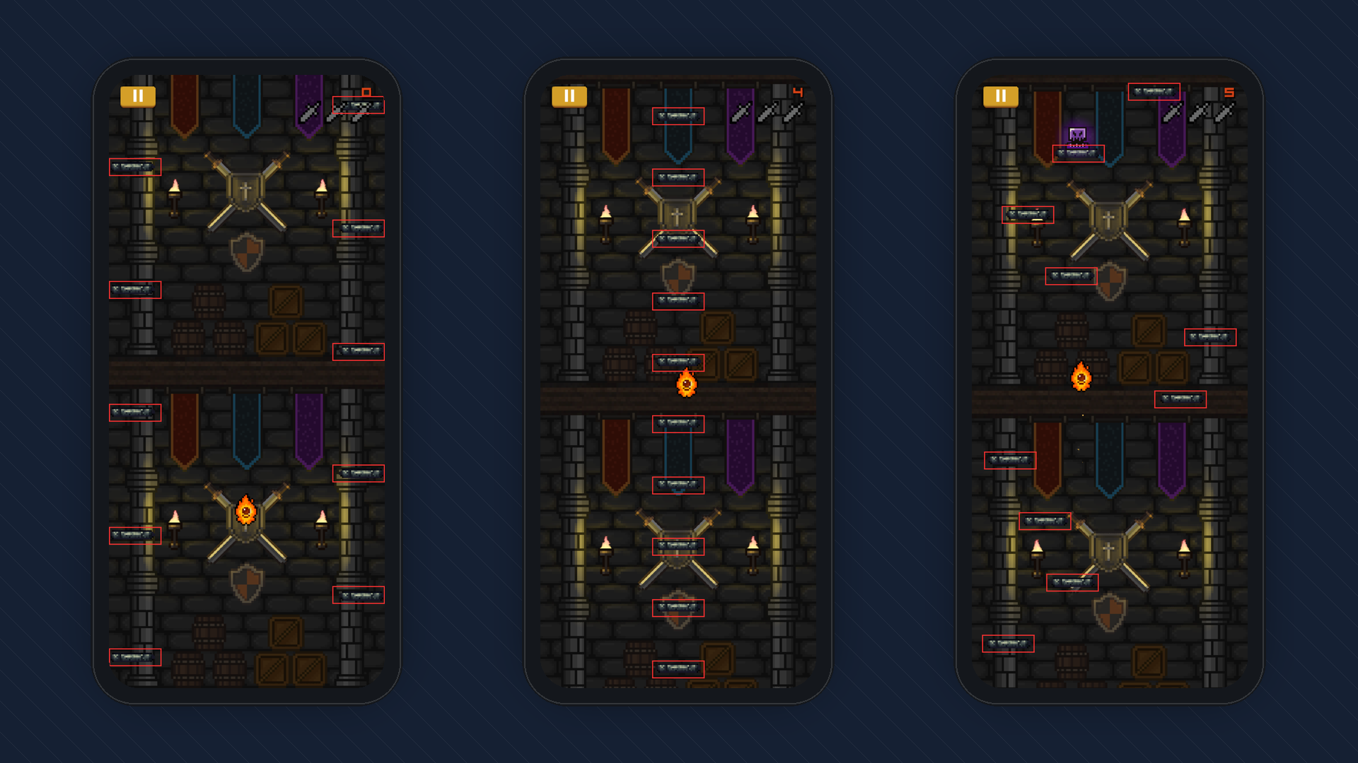
As shown in the figure below, the left case places platforms at opposite extremes, making the game extremely difficult. In the middle case, all platforms share the same horizontal position, so the player can ascend without moving, trivializing the challenge. The right case reflects the distribution players expect. However, with naive uniform sampling, all three outcomes are equally likely, which is undesirable.

There are two ways to address this. One is to author many prefab patterns that share fixed entry and exit positions. This approach demands substantial memory to avoid repetition, and large pattern blocks can cause frame-time spikes when all platforms in a block are instantiated in a single tick. A better alternative is conditioned (constraint-aware) sampling: generate each platform position from a distribution that depends on prior placements, which reduces pathological cases while preserving variety.

Gaussian Distribution

The initial design is using a Gaussian Distribution to determine platform placement, with the mean set at the position of the previous platform. The variance increases via a predefined schedule to ramp game difficulty. Using Box–Muller transform to sample from standard gaussian distribution then later shifted and scaled based on the desired mean and variance to fit the intended distribution.

where $U_1, U_2 \sim \mathrm{Uniform}(0,1)$.

Despite its simplicity, plain Gaussian sampling can quickly place platforms beyond the viewport bounds.

Clamped Gaussian Distribution

Values that fall outside the desired range are clamped to the nearest boundary, resulting in an accumulation of probability mass at the edges. This effect becomes particularly noticeable when the previous platform's position is near the viewport boundary.

Rejection Sampling

Iteratively draw from the predefined distribution, rejecting invalid samples until a valid one appears. Consequently, the operation is not guaranteed to be constant-time.

Truncated Gaussian Distribution

The random variable here is the platform’s horizontal position. Its distribution is truncated Gaussian (normal). To sample from a truncated Gaussian, Box-Muller transform is no longer applicable. Instead, use the cumulative distribution to sample from the truncated Gaussian (normal), which is equivalent to sampling a restricted domain $[a,b]$ of a Gaussian Distribution and renormalize the remaining probability mass.

1. Compute the cumulative probability of the boundary positions, $\mathrm{CDF}(a)$ and $\mathrm{CDF}(b)$.
2. Draw $u \sim \mathrm{Uniform}(\mathrm{CDF}(a), \mathrm{CDF}(b))$, which implicitly renormalize the distribution.
3. $\mathrm{CDF^{-1}}(u)$ is the next platforms position and is guaranteed to be between $a$ and $b$.

Both Gaussian CDF and inverse Gaussian CDF is involved in the sampling of a Truncated Gaussian Distribution. However, Gaussian CDF does not have a closed form expression. Thus, use approximation to calculate the value of the Gaussian CDF and inverse Gaussian CDF.

1. Maclaurin Series: Accurate near 0 only. Ineffective as screen width typically span hundreds of pixels
2. Taylor Series: Requires storing numerous reference points, making it less flexible.

Hence, neither Maclaurin Series nor Taylor Series is suitable to approximate the value of the Gaussian CDF or inverse Gaussian CDF.

To efficiently calculate the value of Gaussian CDF and inverse Gaussian CDF. I first express the CDF in terms of Error Function $\mathrm{erf}$. Then, I can easily use Abramowitz & Stegun Approximation to calculate the value of Error Function in constant time and constant space. And Winitzki Approximation to calculate the value of inverse Error Function in constant time and constant space.

To compute the Gaussian CDF and its inverse efficiently, I first rewrite the CDF using the error function:$\Phi(0,1;x) = \frac{1}{2} + \frac{1}{2} \cdot \mathrm{erf} \left( \frac{x}{\sqrt{2}} \right)$. This also gives$\; \Phi^{-1}(0,1;p) = \sqrt{2} \, \mathrm{erf^{-1}} \! \left( 2p-1 \right)$.

where $\mathrm{erf}(x) = \frac{1}{\sqrt{\pi}}\int_{-x}^{x} e^{-t^{2}}\,dt$.

I then evaluate $\mathrm{erf}$ with the Abramowitz & Stegun Approximation, a fast fixed-cost rational/exponential approximation, and use Winitzki Approximation to evaluate $\mathrm{erf}^{-1}$, which likewise runs in constant time and space.

Despite truncated Gaussian Distribution is effective numerically, it results in cluster near the previous platform which leads to undesirable for game feel.

Weighted Bimodal Truncated Gaussian

To reduce the likelihood of consecutive platforms appearing in the same position, replace the truncated Gaussian Distribution with Bimodal Truncated Gaussian Distribution to determine each new platform's location. The weighting of the two Gaussian components is dynamically adjusted based on the previous platform's position

For instance:

• If the previous platform is centered on the screen, both the left and right Gaussian components are equally weighted.
• If the previous platform is positioned at the first quartile from the left edge, the left Gaussian is assigned a weight of 25%, while the right Gaussian receives a 75% weight.

Weighted Bimodal Truncated Gaussian with Dead Zone

To prevent situations where two consecutive platforms are so close horizontally that the treasure on the lower platform becomes unreachable, I add a dead zone to the position sampling to avoid this.